Why LLMs Behave the Way They Do
An overview of the development of language models.
Background
The key challenge for language modelling has always been capturing meaning. A language model needs to understand not only which words appear in a sentence, but what each word means in the given context. To understand how contemporary language models do this, it helps to understand how they evolved.
From N-grams to Embeddings
Early models, like n-grams, represented words as a set of discrete combinations. They worked by splitting sentences into sequences of \(n\) adjacent symbols, where the next word depends on the previous \(n-1\) words. This dependence on position does not capture the fact that words like rug and carpet have related meanings. As the number of possible n-grams grows rapidly with vocabulary size, this leads to sharp limitations for memory usage and generalisation [1].
A major shift occurred with the introduction of neural network language models by Yoshua Bengio et al in 2003 [2]. Instead of representing words as discrete symbols, neural models represent them as continuous vectors known as word embeddings. Words appearing in similar contexts develop similar vector representations, allowing models to capture semantic relationships between terms. Unlike discrete n-gram models, continuous vector spaces remove the need to explicitly enumerate all possible word combinations. This enables neural networks to learn complex, non-linear relationships between words that traditional count-based approaches cannot represent.
Subsequent advances improved the quality of these embeddings. Models such as Word2Vec [3] and GloVe [4] produced vector representations that captured meaningful semantic relationships between words. A well-known example is the vector analogy king − man + woman ≈ queen, demonstrating that embedding spaces can encode interpretable relationships. The ability to automatically infer semantic structure from large text corpora generated widespread interest in neural language models [5].
![A 2D visualisation of clustering for related words using static word embeddings. Adapted from Tshitoyan et al. [Tshitoyan2019]](/theory-article/Word2Vec%20for%20materials%20properties.png)
Contextual Dependencies
These word vectors had one key problem. They captured the meaning of the word with a static vector, which didn't change depending on surrounding words. But the meaning of each word is fungible depending on its context. For example, "cell" could be refer to a biological cell, a battery cell, or a prison cell- and a static word embedding would represent all of the above as a single vector.
To understand how a word's meaning depends on its context, we model both local and long-range dependencies. Local dependencies are intuitive: we examine the surrounding words within the same sentence or paragraph to infer meaning. Long-range dependencies are less obvious. Here, we consider how each word relates to the broader structure of the document. For example, does a document that ends with a formal conclusion tend to use more formal language throughout? Are there other subtle patterns that a computer could learn from vast amounts of statistical data, patterns that would never be apparent to a human reader? In essence, the goal is to leverage as much contextual information as possible to determine meaning.
Recurrent Neural Networks
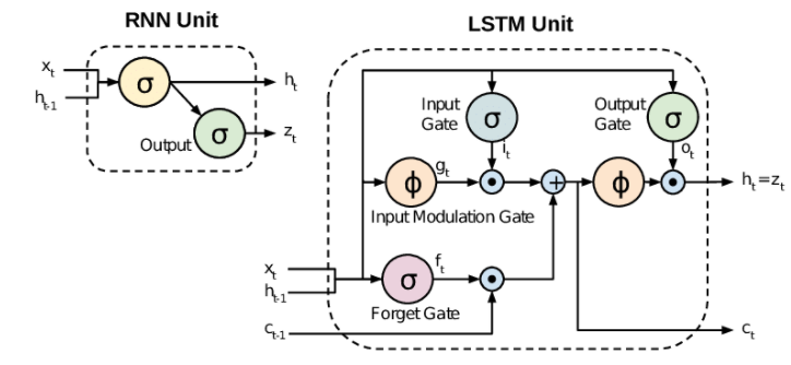
To capture sequential dependencies in language, Recurrent Neural Networks (RNNs) process tokens sequentially while maintaining a hidden state that carries information from earlier words. This hidden state enables later tokens to be interpreted in context. Later models leveraged these contextual hidden states to produce contextual word representations, such as ELMo.
During training, gradients are propagated backward through time and repeatedly interact with the same weights at each step. When these values are small, the gradients progressively shrink, leading to the vanishing gradient problem, where the model gradually loses information from earlier tokens. When the values are large, the gradients rapidly grow, resulting in exploding gradients, which cause unstable parameter updates and can make training diverge [11].
The LSTM
Long Short-Term Memory (LSTM) networks mitigate the exploding gradient issues for RNNs using gating mechanisms to selectively retain information [8].
The LSTM-based Embeddings from Language Model (ELMo) [10] demonstrated that RNNs could produce genuinely contextual word embeddings, where the same word receives different representations depending on its surrounding context. This directly addressed the polysemy problem that had limited all prior approaches, and contextual embeddings became the new state of the art for language modelling. LSTM architectures also do not scale well due to the computational cost of managing hidden states across many layers [11].
Attention mechanisms were first introduced to address some of the limitations of RNNs in tasks like machine translation [12]. This idea was extended in the paper "Attention is All You Need", which discarded RNN architectures entirely, in favour of using self-attention to compute input and output representations [13]. Transformer-based architectures, such as BERT [14] and GPT-2 [15], have demonstrated significant performance improvements over RNN models in language modelling [16]. The key advantage of Transformer models arises from their ability to be trained non-sequentially. This has allowed us to scale the size and performance of these models from toys to sophisticated general purpose machines capable of providing an approximate solution to almost any question. As a result of these architectural advantages, Transformers have widely eclipsed LSTMs in practice.
Tokenization
In order to utilise text as input in LMs, it must first be converted into tokens. This process is handled by a tokenizer. Text is first normalised, removing elements not expected by the tokenizer, such as accents or non-ASCII characters. It is then split into sentences, and tokens are assigned to the contents. Tokens may represent words, parts of words, or individual characters.
![An example of sentence splitting and tokenization using the BERT tokenizer. Adapted from Huang et al. [huang_cole_2022]](/theory-article/tokenization.png)
The embedding matrix contains the vectors used to represent tokens. The number of model parameters contributed by this matrix is the vocabulary size multiplied by the dimensions of the word embeddings.
Out-of-vocabulary words are represented by the [UNKNOWN] token, which can lead to a large loss of information. Therefore, it is important that our vocabulary is able to represent as many word as possible.
If tokenization occurred at the word-level, every unique word would have its own token. This vocabulary would have to include all common permutations of casing and punctuation to avoid out-of-vocabulary words, and would result in an extremely large vocabulary size.
If tokenization occurred at the character level, each individual character would be a unique token. While this would produce a small vocabulary size, it would introduce challenges like poor model convergence and higher training cost, as the semantic meaning of words is completely lost.
Subword Tokenization
Subword tokenization algorithms work on the principle that frequently used words should not be split into smaller subwords, so that their full semantic meaning can be more accurately represented. However, rare words should be broken down into meaningful subwords. To summarise, a vocabulary must balance the ability to capture semantic meaning with a limited vocabulary size.
In addition to learned tokens, there are special token included in the vocabulary. For example, in BERT, the token ID of 101 represents the beginning of a sequence, 102 represents the end of a sequence, and 0 represents padding. Special tokens are also added for specific tasks, such as the [MASK] token used in masked language modelling.
Vocabulary creation
A tokenizer vocabulary can be created through various algorithmic approaches, including Byte-Pair Encoding (BPE) [19] and WordPiece [20]. The objective is to create the best vocabulary to represent a given corpus of language with as few tokens as possible.
In Byte-Pair Encoding, the initial vocabulary consists of individual characters. The algorithm repeatedly identifies the most frequent pair of adjacent tokens in the corpus and merges them into a new token. This iterative merging process continues until the desired vocabulary size is reached.
In WordPiece, the vocabulary also begins with individual characters, but token merges are selected using a probabilistic objective and potential token merges are evaluated based on how much they increase the likelihood of the data. The merge that most improves the corpus likelihood is added to the vocabulary, and this process continues until the target vocabulary size is achieved.
Because WordPiece selects merges based on likelihood improvements rather than raw frequency alone, it typically produces a more representative and generalisable subword vocabulary [21]
WordPiece generally produces better results than BPE [21], so it is preferred for vocabulary creation.
Subword tokenization enables the model to process words it has never seen before by breaking them into subwords. This leads to a large reduction in the use of the [UNKNOWN] token, and loss of information. In BERT's WordPiece tokenization, the end of a word is marked with ##. For example, tokenization is split into the "token" and "##ization" tokens. Every token in the vocabulary is mapped to a unique identifier (ID). This means that tokenizers from different models cannot usually be used interchangeably.
When token IDs are assigned, an attention mask is also created. This mask indicates which tokens should be attended to and which are padding. Padding tokens are used to ensure that all input sequences are of the same length, allowing for efficient processing as rectangular tensors. The attention mask ensures the model ignores padding tokens during calculations.
Token Embeddings
Each token is converted into a vector by combining three different types of embeddings: token, position, and segment embeddings. Each token ID corresponds to a row in the embedding matrix, representing the token's dense vector embedding. Position embeddings encode each token's location in the input sequence, as Transformer models lack other mechanisms for resolving positional information, such as the hidden states found in RNNs. Segment embeddings distinguish different parts of the input, such as sentence boundaries.
![Assignment of embeddings to tokens in BERT. Adapted from Devlin et al. [devlin2019bert]](/theory-article/BERTtokenization.png)
It is possible to compare the similarity of words using their token embeddings. Each embedding is a vector and as a result a simple cosine similarity comparison can be used to quickly measure how similar any two embeddings are.
Transformer Model Architecture
![The architecture of the Transformer model. Adapted from Vaswani et al. [vaswani2023attentionneed]](/theory-article/TransformerArchitecture.png)
The Encoder
In the Transformer model, the encoder maps an input sequence of symbols \((x_1, \dots, x_n)\) into a sequence of continuous representations \(\mathbf{z} = (z_1, \dots, z_n)\). The decoder then generates an output sequence \((y_1, \dots, y_m)\) of symbols one element at a time, based on the encoded representations \(\mathbf{z}\).
An attention function maps a query and a set of key-value pairs to an output, where the query, keys, values, and output are all vectors. The output is computed as a weighted sum of the values, where the weights are determined by the compatibility of the query with the corresponding key.
Scaled Dot-Product Attention
While general attention mechanisms establish dependencies between different elements of embeddings, self-attention computes dependencies within a single sequence. The encoder block in Transformers employs self-attention, specifically "Scaled Dot-Product Attention."
![The composition of Scaled Dot-Product Attention and Multi-Headed Attention. Adapted from Vaswani et al. [vaswani2023attentionneed]](/theory-article/AttentionHeads.png)
Input tokens are first embedded into vectors and processed by a series of blocks. In each block, the input is linearly transformed into three matrices: Query (Q), Key (K), and Value (V).
Attention in the Transformer is multi-headed, meaning multiple attention mechanisms (heads) are applied in parallel. Each head processes a different subspace of Q, K, and V, enabling the model to capture various types of dependencies between tokens, both long-term and short-term.
The input consists of queries and keys of dimension \(d_k\), and values of dimension \(d_v\). Inside each head, attention scores are computed simultaneously for a set of queries, packed together into a matrix \(\mathbf{Q}\). The keys and values are similarly packed into matrices \(\mathbf{K}\) and \(\mathbf{V}\). The output of each head is computed as:
Here, the softmax function is applied row-wise to compute the attention probabilities, which are used to weigh the values \(\mathbf{V}\). The softmax function amplifies the scores of highly related token pairs, making their relationships more prominent. For large values of \(d_k\), the softmax function has extremely small gradients, so the product is scaled by \(\frac{1}{\sqrt{d_k}}\).
The resulting attention probabilities capture the syntactic and semantic properties of tokens, which can be compared directly. The attention output is then combined with the block input via a residual connection, followed by layer normalisation.
Q, K, and V are processed by attention to get the intermediate features, the output of the attention. A residual layer then adds the attention output with the block input and performs layer normalisation.
Multi-Head Attention
Multi-Head Attention is defined by the following equations:
Where the output of every attention head in the index, \(\text{head}_i\), is computed as described in Equation 1, and the projections are parameter matrices \(W_i^Q\), \(W_i^K\), \(W_i^V\), and \(W^O\).
Following the multi-head attention mechanism, a feed-forward network is applied, which consists of two fully connected layers with a non-linear activation function in between. After this, another residual connection and layer normalisation are applied, resulting in the block's output. This block structure can be repeated multiple times.
The Decoder
We modify the self-attention sub-layer in the decoder stack, to prevent positions from attending to subsequent positions, through the use of a masking mechanism. This ensures that the decoder computes attention scores for the sequence, only up to and including the current position. The output of each attention head is concatenated and linearly transformed as described in Equation 3.
Similar to the encoder, we employ residual connections around each of the sub-layers, meaning the output of the self-attention sub-layer is added to the original input of this sub-layer, followed by layer normalisation [13]. This step helps to stabilise training.
Cross-Attention
In, "cross-attention", the source of keys and values is different from that of queries. The query is taken from the previous layer's output (the decoder's self-attention) whereas the keys and values come from the encoder's output, as can be seen in Figure 5. The attention output is computed in a way such that the decoder focuses on relevant parts of the encoded input sequence whilst generating new tokens.
Again, between layers, residual connection and layer normalisation is applied. Similarly to the end of the encoder block, a feed-forward network is applied. Afterwards, a final stage of residual connection and layer normalisation is applied.
The final decoder output is a set of vectors corresponding to a position in the output sequence. These vectors pass through a linear transformation (matrix multiplication with learnt weights) to map them to the total vocabulary size. This output is equivalent to a score for each word.
The softmax function is then applied to convert the word scores into a probability. The best word for each position is interpreted as the maximum of the output of the softmax layer, and is generated as the next word in the output sequence. One token is generated a time in an autoregressive manner. Each generated token is fed back into the decoder to predict the next token, until the end-of-sequence token is generated.
Fundamental limitations
Transformers do not parse tokens sequentially. While this allows all tokens in a sequence to be processed simultaneously, it makes it challenging to capture the positional relationships between tokens. Transformers capture positional information by using position embeddings, however this positional encoding is not further refined during training [22] [23].
The attention mechanism enables Transformer models to capture long-range dependencies between tokens. More dependencies can be captured by increasing the number of attention heads, layers, and model parameters. However, self-attention can lead to an overemphasis on global dependencies at the expense of valuable local context, making the models less effective at capturing localised linguistic patterns [24] [25].
Computational Cost and Hallucinations
Because the attention mechanism scales quadratically with sequence length, applying Transformers to long sequences is computationally expensive. Utilising a very long context window requires the adaptation of techniques such as rotary position embeddings [26]. Additionally, Transformers require large amounts of data to acquire accurate representations, and the logic used by Transformers is not easy to interpret, posing challenges for experimentation and deployment.
Transformers assign confidence scores using the model's estimated likelihood of that prediction given the learned statistical patterns in the training data. During sequence generation, this process occurs step-by-step, allowing token-level probabilities to be fused into a sentence or paragraph-level confidence score. However, these scores do not necessarily reflect true certainty. They measure internal consistency within the model's learned distribution rather than factual correctness. Consequently, Transformers may assign high confidence to incorrect or fabricated outputs, particularly in cases where the model generates plausible but unsupported information (hallucinations) [57].
Encoder-Only Models
Encoder-only models focus on understanding input data to make predictions. They are commonly used for discriminative tasks such as NER and RE.
The block structure of the encoder in the Transformer architecture can be repeated multiple times. Each encoder block contains a multi-head attention layer and a feed-forward layer, with residual connections and layer normalisation at every stage. The output of the final block is fed into a classification layer to produce a prediction. When using multiple encoder blocks in series, each block processes the output of the previous one. Stacking multiple encoder blocks improves the model's ability to map complex token dependencies.
The BERT paper used an encoder-only structure, experimenting with different numbers of layers, hidden units, and attention heads. They published bert-base-uncased (12 layers, 768 hidden states, 12 attention heads, 110M parameters) and bert-large-uncased (24 layers, 1024-hidden states, 16 attention heads, 336M parameters). Model ablations are shown in Table 1.
| #L | #H | #A | LM (ppl) | MNLI-m | MRPC | SST-2 |
|---|---|---|---|---|---|---|
| 3 | 768 | 12 | 5.84 | 77.9 | 79.8 | 88.4 |
| 6 | 768 | 3 | 5.24 | 80.6 | 82.2 | 90.7 |
| 6 | 768 | 12 | 4.68 | 81.9 | 84.8 | 91.3 |
| 12 | 768 | 12 | 3.99 | 84.4 | 86.7 | 92.9 |
| 12 | 1024 | 16 | 3.54 | 85.7 | 86.9 | 93.3 |
| 24 | 1024 | 16 | 3.23 | 86.6 | 87.8 | 93.7 |
Table 1. Accuracy scores for different BERT ablations on the MNLI-m, MRPC and SST-2 datasets. #L is the number of layers, #H the hidden size, #A the number of heads and "LM (ppl)" the perplexity of masked training data. Adapted from Devlin et al. [14]
BERT learns language bi-directionally. The motivation for this is that for token-level tasks such as question answering, it is crucial to incorporate context from both directions [27]. This is better captured by a bi-directional approach, compared to a left-to-right approach, due to the positional dependence of the attention mechanism [14].
![A comparison of feature generation in BERT, GPT, and ELMo, highlighting BERT's use of a bi-directional approach. Adapted from Devlin et al. [devlin2019bert]](/theory-article/BERTconditioning.png)
BERT is a bi-directional model. As it can view neighbouring tokens in both directions, it requires a different training approach to a sequential, left-to-right model. Masked Language Modelling (MLM) is therefore implemented, which involves randomly masking 15% of the input tokens by replacing them with the [MASK] token. The transformer attempts to guess what word has been masked by using multiple attention heads to interpret token dependencies.
BERT was trained on both MLM and Next Sentence Prediction (NSP), though later models found pre-training on the NSP task unnecessary [28].
![The pre-training and fine-tuning procedures for BERT, an encoder-only model. Adapted from Devlin et al. [devlin2019bert]](/theory-article/BERT.png)
Decoder-Only Models
Decoder-only models focus on generating sequences based on preceding context. They are often used for for autoregressive text generation tasks. Examples of text generation tasks include machine translation and text summarisation. The principles behind stacking multiple decoder blocks or encoder blocks in series are the same.
In the Decoder, the self-attention mechanism is applied sequentially. The generation of each successive word in the output sequence depends on the previously generated words. A sequential operation ensures that the Decoder generates words one at a time in the correct order.
Decoder-only architectures are highly capable [29], but not the first choice of model architecture to utilise for discriminative tasks.
Model Optimisation
Fine-Tuning
After pre-training, a language model can be fine-tuned for a specific purpose by adding a task-specific output layer on top of the pre-trained model.
Fine-tuning often involves training only this new layer on task-specific data, whilst keeping all other layers unchanged (or frozen). Alternatively, the entire model can be fine-tuned, although this can actually degrade overall model performance via effects like catastrophic forgetting [31] [32] [33].
![A visualisation of the model loss when pre-training and fine-tuning a language model on different datasets. Adapted from Hao et al. [hao2019visualizing]](/theory-article/Loss-surfaces.png)
Parameter-Efficient Techniques
Balancing training cost, performance improvement, and the impact on overall model behaviour is a complex task. As a result, a variety of techniques have been created, including adapter modules [34] and Parameter-Efficient Fine Tuning (PEFT) methods [35][36].
Fine-tuning can be lead to performance improvements, even when applied with a small dataset. For example, performance on QA tasks can be significantly improved achieved with as few as 300 high quality, labelled examples [37].
Domain-Specific Models
Since we can only go so far by fine-tuning a model, we might pre-train a model where we have a stronger bias towards a particular domain in the training corpus. Since the writing style and terminology used by each domain is different, such as scientific papers which include symbols, and the model can learn more specialised representations [33] [38].
Furthermore, we might adjust the vocabulary used by the model (the tokenizer). Rather than optimising our tokenizer to represent a very wide combination of words using many sub-tokens, we could bias it towards representing larger tokens more strongly.
This has led researchers to create the likes of SciBERT [39], BioBERT [40] and Med-BERT [41], MatSciBERT [42], and MatBERT [43] for slightly better domain-specific performance. From the development of domain-specific models, we can infer rules about efficient hyperparameter selection, corpus curation, and efficient model inference.
Model Optimisation Strategies
We are able to make very large transformer-based language models. Various optimisation techniques allow us to make models which are roughly as performant, but much smaller. The logic behind this is that various neurons have higher importance in decision making than others. A straightforwards method of resolving this is ablation. Ablation involves systematically removing or modifying components of a language model to measure the resulting impact on overall performance [44].
Pruning
Model ablation removes components of a model to analyze their impact on performance, whereas model pruning removes unnecessary weights or neurons to reduce model size and improve efficiency. Model Pruning reduces the size and complexity of a model by removing less important parameters. This can be done through structured approaches, such as network slimming [45], or unstructured approaches, such as magnitude-based pruning [46]. While pruning effectively reduces model size, it it often results in irregular sparsity patterns that hardware may not efficiently exploit, leading to limited performance improvements [47].
Knowledge Distillation
Knowledge Distillation involves using a larger "teacher" model to guide the learning process of a smaller "student" model [48]. This technique is relatively straightforward to implement, and has shown promising experimental results. For example, Distil-BERT achieves 97% of BERT's performance on benchmarks while using 40% less memory [49]. However, this approach incurs the additional computational cost of training both the teacher and student models, which can be significant, especially if the teacher model is substantially larger.
![The teacher-student framework used in knowledge distillation. Adapted from Gou et al. [gou2021knowledge]](/theory-article/KD.png)
Low-rank factorisation methods decompose large matrices, such as those representing model weights, into products of smaller matrices [51]. Techniques like tensor decomposition [52] reduce the number of parameters by assuming that data can be well-represented by low-rank matrices. However, this assumption may not always hold true, particularly for NLP, potentially leading to model bias and reduced performance.
Quantisation and Parameter Sharing
Model Quantisation reduces the precision of numbers used to represent model parameters (for example, reducing 32-bit floating-point to 8-bit or 4-bit integers). This approach significantly decreases memory usage and computational demands. Quantisation can be applied post-training or during training itself [53]. However, if not carefully implemented, quantisation can result in significant accuracy loss.
Parameter Sharing involves sharing weights across different parts of the model, such as across layers or attention heads [54]. This technique reduces the total number of parameters while sometimes even enhancing model performance due to implicit regularisation effects [55]. However, it can also alter the behaviour of the model in unexpected ways.
Certain model optimisation strategies can be applied in a complementary fashion, such as combining knowledge distillation with quantisation [56]. Strategies should be selected based on ease of implementation, the size of the model being used, and the specific training task.
Bibliography
- Kneser, Reinhard, Ney, Hermann. Improved backing-off for m-gram language modeling. 1995 international conference on acoustics, speech, and signal processing, 1995. DOI: 10.1109/ICASSP.1995.479394
- Bengio, Yoshua, Ducharme, Réjean, Vincent, Pascal. A neural probabilistic language model. Journal of Machine Learning Research, 2003. URL: https://www.jmlr.org/papers/volume3/bengio03a/bengio03a.pdf
- Tomas Mikolov, Kai Chen, Greg Corrado, Jeffrey Dean. Efficient Estimation of Word Representations in Vector Space. arXiv, 2013. DOI: 10.48550/arXiv.1301.3781
- Pennington, Jeffrey, Socher, Richard, Manning, Christopher. GloVe: Global Vectors for Word Representation. Proceedings of the 2014 Conference on Empirical Methods in Natural Language Processing (EMNLP), 2014. DOI: 10.3115/v1/D14-1162
- Tshitoyan, Vahe, Dagdelen, John, Weston, Leigh, Dunn, Alexander, Rong, Ziqin, Kononova, Olga, Persson, Kristin A., Ceder, Gerbrand, Jain, Anubhav. Unsupervised word embeddings capture latent knowledge from materials science literature. Nature, 2019. DOI: 10.1038/s41586-019-1335-8
- LeCun, Yann, Bengio, Yoshua, Hinton, Geoffrey. Deep learning. nature, 2015. DOI: 10.1038/nature14539
- Pascanu, Razvan, Mikolov, Tomas, Bengio, Yoshua. On the difficulty of training recurrent neural networks. International conference on machine learning, 2013. DOI: 10.48550/arXiv.1211.5063
- Hochreiter, Sepp, Schmidhuber, Jürgen. Long short-term memory. Neural computation, 1997. DOI: 10.1162/neco.1997.9.8.1735
- Szelogowski, Daniel James. Deep learning for musical form: recognition and analysis. University of Wisconsin-Whitewater, 2022. DOI: 10.31237/osf.io/ts27q
- Peters, Matthew E., Neumann, Mark, Iyyer, Mohit, Gardner, Matt, Clark, Christopher, Lee, Kenton, Zettlemoyer, Luke. Deep Contextualized Word Representations. Proceedings of the 2018 Conference of the North American Chapter of the Association for Computational Linguistics: Human Language Technologies, Volume 1 (Long Papers), 2018. DOI: 10.18653/v1/N18-1202
- Tang, Gongbo, Müller, Mathias, Rios, Annette, Sennrich, Rico. Why Self-Attention A Targeted Evaluation of Neural Machine Translation Architectures. Proceedings of the 2018 Conference on Empirical Methods in Natural Language Processing, 2018. DOI: 10.18653/v1/D18-1458
- Bahdanau, Dzmitry, Cho, Kyunghyun, Bengio, Yoshua. Neural machine translation by jointly learning to align and translate. arXiv, 2014. DOI: 10.48550/arXiv.1409.0473
- Ashish Vaswani, Noam Shazeer, Niki Parmar, Jakob Uszkoreit, Llion Jones, Aidan N. Gomez, Lukasz Kaiser, Illia Polosukhin. Attention Is All You Need. arXiv, 2023. DOI: 10.48550/arXiv.1706.03762
- Jacob Devlin, Ming-Wei Chang, Kenton Lee, Kristina Toutanova. BERT: Pre-training of Deep Bidirectional Transformers for Language Understanding. arXiv, 2019. DOI: 10.48550/arXiv.1810.04805
- Radford, Alec, Wu, Jeffrey, Child, Rewon, Luan, David, Amodei, Dario, Sutskever, Ilya, others. Language models are unsupervised multitask learners. OpenAI blog, 2019. URL: https://cdn.openai.com/better-language-models/language_models_are_unsupervised_multitask_learners.pdf
- Rebecca Marvin, Tal Linzen. Targeted Syntactic Evaluation of Language Models. arXiv, 2018. DOI: 10.48550/arXiv.1808.09031
- Paul Bilokon, Yitao Qiu. Transformers versus LSTMs for electronic trading. arXiv, 2023. DOI: 10.48550/arXiv.2309.11400
- Huang, Shun-Wei, Cole, Jacqueline M.. BatteryDataExtractor: battery-aware text-mining software embedded with BERT models. 2022. DOI: 10.1039/d2sc04322j
- Sennrich, Rico, Haddow, Barry, Birch, Alexandra. Neural machine translation of rare words with subword units. arXiv, 2015. DOI: 10.48550/arXiv.1508.07909
- Schuster, Mike, Nakajima, Kaisuke. Japanese and korean voice search. 2012 IEEE international conference on acoustics, speech and signal processing (ICASSP), 2012. DOI: 10.1109/icassp.2012.6289079
- Bostrom, Kaj, Durrett, Greg. Byte pair encoding is suboptimal for language model pretraining. arXiv, 2020. DOI: 10.48550/arXiv.2004.03720
- Xiangxiang Chu, Zhi Tian, Bo Zhang, Xinlong Wang, Chunhua Shen. Conditional Positional Encodings for Vision Transformers. arXiv, 2023. DOI: 10.48550/arXiv.2102.10882
- Pu-Chin Chen, Henry Tsai, Srinadh Bhojanapalli, Hyung Won Chung, Yin-Wen Chang, Chun-Sung Ferng. A Simple and Effective Positional Encoding for Transformers. arXiv, 2021. DOI: 10.48550/arXiv.2104.08698
- Baosong Yang, Zhaopeng Tu, Derek F. Wong, Fandong Meng, Lidia S. Chao, Tong Zhang. Modeling Localness for Self-Attention Networks. arXiv, 2018. DOI: 10.48550/arXiv.1810.10182
- Baosong Yang, Longyue Wang, Derek F. Wong, Shuming Shi, Zhaopeng Tu. Context-aware Self-Attention Networks for Natural Language Processing. Neurocomputing, 2021. DOI: https://doi.org/10.1016/j.neucom.2021.06.009
- Jianlin Su, Yu Lu, Shengfeng Pan, Ahmed Murtadha, Bo Wen, Yunfeng Liu. RoFormer: Enhanced Transformer with Rotary Position Embedding. arXiv, 2023. DOI: 10.48550/arXiv.2104.09864
- Shreyashree, S, Sunagar, Pramod, Rajarajeswari, S, Kanavalli, Anita. A literature review on bidirectional encoder representations from transformers. Inventive Computation and Information Technologies: Proceedings of ICICIT 2021, 2022. DOI: 10.1007/978-981-16-6723-7_23
- Yinhan Liu, Myle Ott, Naman Goyal, Jingfei Du, Mandar Joshi, Danqi Chen, Omer Levy, Mike Lewis, Luke Zettlemoyer, Veselin Stoyanov. RoBERTa: A Robustly Optimized BERT Pretraining Approach. CoRR, 2019. DOI: 10.48550/arXiv.1907.11692
- Roberts, Jesse. How Powerful are Decoder-Only Transformer Neural Models. arXiv, 2023. DOI: 10.48550/arXiv.2305.17026
- Hao, Yaru, Dong, Li, Wei, Furu, Xu, Ke. Visualizing and understanding the effectiveness of BERT. arXiv, 2019. DOI: 10.48550/arXiv.1908.05620
- Suchin Gururangan, Ana Marasovic, Swabha Swayamdipta, Kyle Lo, Iz Beltagy, Doug Downey, Noah A. Smith. Don't Stop Pretraining: Adapt Language Models to Domains and Tasks. arXiv, 2020. DOI: 10.48550/arXiv.2004.10964
- Vrbancic, Grega, Podgorelec, Vili. Transfer learning with adaptive fine-tuning. IEEE Access, 2020. DOI: 10.1109/access.2020.3034343
- Hong, Zhi, Ward, Logan, Chard, Kyle, Blaiszik, Ben, Foster, Ian. Challenges and Advances in Information Extraction from Scientific Literature: a Review. JOM, 2021. DOI: 10.1007/s11837-021-04902-9
- Houlsby, Neil, Giurgiu, Andrei, Jastrzebski, Stanislaw, Morrone, Bruna, De Laroussilhe, Quentin, Gesmundo, Andrea, Attariyan, Mona, Gelly, Sylvain. Parameter-Efficient Transfer Learning for NLP. Proceedings of the 36th International Conference on Machine Learning, 2019. DOI: 10.48550/arXiv.1902.00751
- Ding, Ning, Qin, Yujia, Yang, Guang, Wei, Fuchao, Yang, Zonghan, Su, Yusheng, Hu, Shengding, Chen, Yulin, Chan, Chi-Min, Chen, Weize, others. Parameter-efficient fine-tuning of large-scale pre-trained language models. Nature Machine Intelligence, 2023. DOI: 10.1038/s42256-023-00626-4
- Fu, Zihao, Yang, Haoran, So, Anthony Man-Cho, Lam, Wai, Bing, Lidong, Collier, Nigel. On the effectiveness of parameter-efficient fine-tuning. Proceedings of the AAAI conference on artificial intelligence, 2023. DOI: 10.1609/aaai.v37i11.26505
- Huang, Shu, Cole, Jacqueline M.. BatteryBERT: A Pretrained Language Model for Battery Database Enhancement. Journal of Chemical Information and Modeling, 2022. DOI: 10.1021/acs.jcim.2c00035
- Zhao, Jiuyang, Huang, Shu, Cole, Jacqueline M. OpticalBERT and OpticalTable-SQA: text-and table-based language models for the optical-materials domain. Journal of Chemical Information and Modeling, 2023. DOI: 10.1021/acs.jcim.2c01259
- Iz Beltagy, Kyle Lo, Arman Cohan. SciBERT: A Pretrained Language Model for Scientific Text. arXiv, 2019. DOI: 10.48550/arXiv.1903.10676
- Lee, Jinhyuk, Yoon, Wonjin, Kim, Sungdong, Kim, Donghyeon, Kim, Sunkyu, So, Chan Ho, Kang, Jaewoo. BioBERT: a pre-trained biomedical language representation model for biomedical text mining. Bioinformatics, 2019. DOI: 10.1093/bioinformatics/btz682
- Laila Rasmy, Yang Xiang, Ziqian Xie, Cui Tao, Degui Zhi. Med-BERT: pre-trained contextualized embeddings on large-scale structured electronic health records for disease prediction. arXiv, 2020. DOI: 10.48550/arXiv.2005.12833
- Gupta, Tanishq, Zaki, Mohd, Krishnan, NM Anoop, Mausam. MatSciBERT: A materials domain language model for text mining and information extraction. npj Computational Materials, 2022. DOI: 10.1038/s41524-022-00784-w
- Trewartha, Amalie, Walker, Nicholas, Huo, Haoyan, Lee, Sanghoon, Cruse, Kevin, Dagdelen, John, Dunn, Alexander, Persson, Kristin A, Ceder, Gerbrand, Jain, Anubhav. Quantifying the advantage of domain-specific pre-training on named entity recognition tasks in materials science. Patterns, 2022. DOI: 10.1016/j.patter.2022.100488
- Jackson, Richard G, Jansson, Erik, Lagerberg, Aron, Ford, Elliot, Poroshin, Vladimir, Scrivener, Timothy, Axelsson, Mats, Johansson, Martin, Franco, Lesly Arun, Papa, Eliseo. Ablations over transformer models for biomedical relationship extraction. F1000Research, 2020. DOI: 10.12688/f1000research.24552.1
- Zhuang Liu, Jianguo Li, Zhiqiang Shen, Gao Huang, Shoumeng Yan, Changshui Zhang. Learning Efficient Convolutional Networks through Network Slimming. arXiv, 2017. DOI: 10.48550/arXiv.1708.06519
- Han, Song, Pool, Jeff, Tran, John, Dally, William. Learning both Weights and Connections for Efficient Neural Network. Advances in Neural Information Processing Systems, 2015. DOI: 10.48550/arXiv.1506.02626
- Yin, Lu, Li, Gen, Fang, Meng, Shen, Li, Huang, Tianjin, Wang, Zhangyang, Menkovski, Vlado, Ma, Xiaolong, Pechenizkiy, Mykola, Liu, Shiwei, others. Dynamic sparsity is channel-level sparsity learner. Advances in Neural Information Processing Systems, 2024. DOI: 10.48550/arXiv.2305.19454
- Geoffrey Hinton, Oriol Vinyals, Jeff Dean. Distilling the Knowledge in a Neural Network. arXiv, 2015. DOI: 10.48550/arXiv.1503.02531
- Victor Sanh, Lysandre Debut, Julien Chaumond, Thomas Wolf. DistilBERT, a distilled version of BERT: smaller, faster, cheaper and lighter. arXiv, 2020. DOI: 10.48550/arXiv.1910.01108
- Gou, Jianping, Yu, Baosheng, Maybank, Stephen J, Tao, Dacheng. Knowledge distillation: A survey. International Journal of Computer Vision, 2021. DOI: 10.1007/s11263-021-01453-z
- Yu, Xiyu, Liu, Tongliang, Wang, Xinchao, Tao, Dacheng. On Compressing Deep Models by Low Rank and Sparse Decomposition. 2017 IEEE Conference on Computer Vision and Pattern Recognition (CVPR), 2017. DOI: 10.1109/CVPR.2017.15
- Remi Denton, Wojciech Zaremba, Joan Bruna, Yann LeCun, Rob Fergus. Exploiting Linear Structure Within Convolutional Networks for Efficient Evaluation. arXiv, 2014. DOI: 10.48550/arXiv.1404.0736
- Zhou, Yiren, Moosavi-Dezfooli, Seyed-Mohsen, Cheung, Ngai-Man, Frossard, Pascal. Adaptive quantization for deep neural network. Proceedings of the AAAI Conference on Artificial Intelligence, 2018. DOI: 10.1609/aaai.v32i1.11623
- Lan, Z. Albert: A lite bert for self-supervised learning of language representations. arXiv, 2019. DOI: 10.48550/arXiv.1909.11942
- Takase, Sho, Kiyono, Shun. Lessons on parameter sharing across layers in transformers. arXiv, 2021. DOI: 10.48550/arXiv.2104.06022
- Polino, Antonio, Pascanu, Razvan, Alistarh, Dan. Model compression via distillation and quantization. arXiv, 2018. DOI: 10.48550/arXiv.1802.05668
- Zhang, Yue, Li, Yafu, Cui, Leyang, Cai, Deng, Liu, Lemao, Fu, Tingchen, Huang, Xinting, et al.. Siren's Song in the AI Ocean: A Survey on Hallucination in Large Language Models. arXiv, 2023. DOI: 10.48550/arXiv.2309.01219